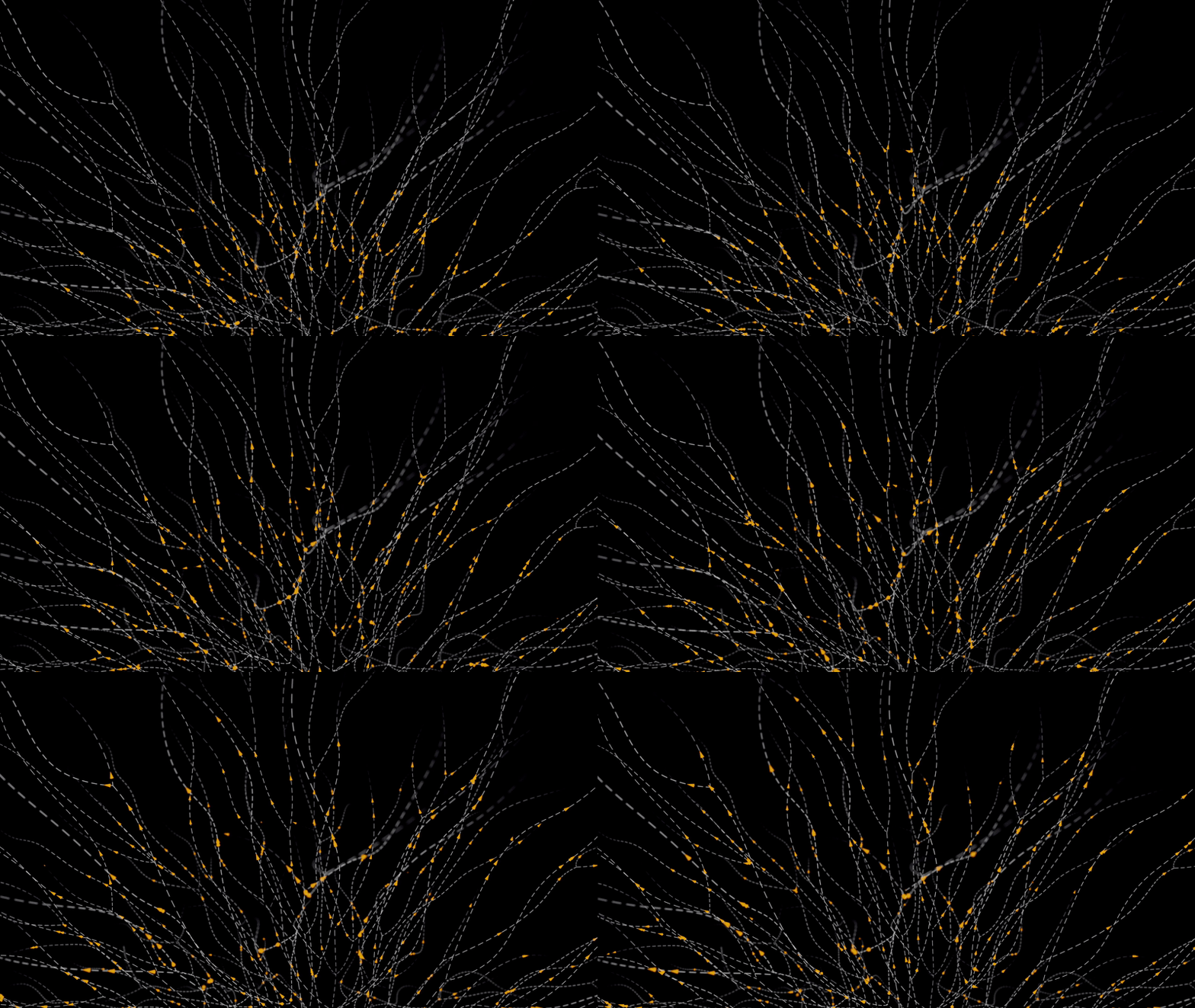
The starting curve network used in this effect is outlined here. It gives us a single root from which the entire network emerges:

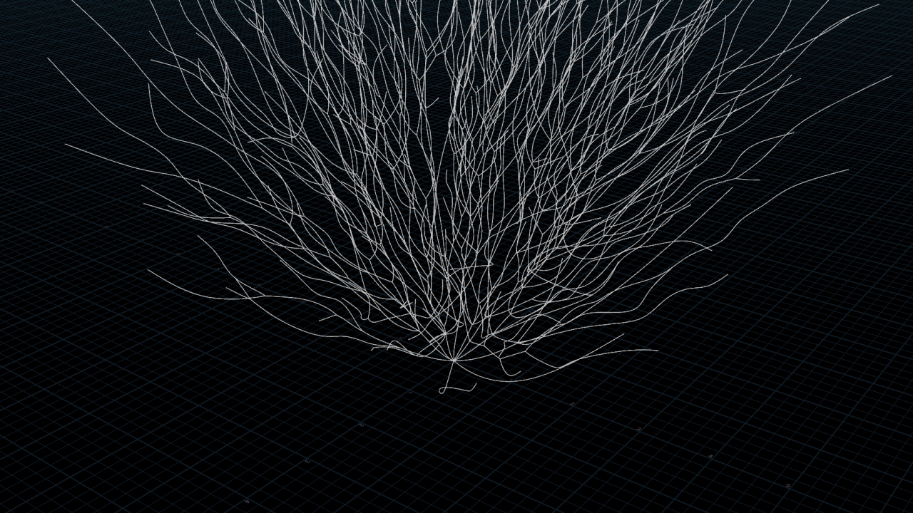
The crux of the effect is to position a particle on a prim with a straightforward VEX function, primuv(). Each prim has an intrinsic set of uvs (with only the U component of relevant to a polyline), giving us a nice normalized range to work with. We can use this range to sample the position (…and potentially other things) at any point along a prim.

Matt Estela has a longer write up of the extremely useful primuv(), here.

With this in mind we can scatter particles onto prims, record the prim on which each particle sits, and then send particles along their prims by sampling with an offset U attrib along the lines of primuv(0, "P", i@sourceprim, v@sourceuv). It’s not unlike what the combo of a ScatterSOP (with sourceprim and sourceprimuv attribs ticked) followed by an AttributeInterpolateSOP might do.

That’s all very well, but what happens when we reach the end of the prim we’ve been travelling along? We need to pick a new one.

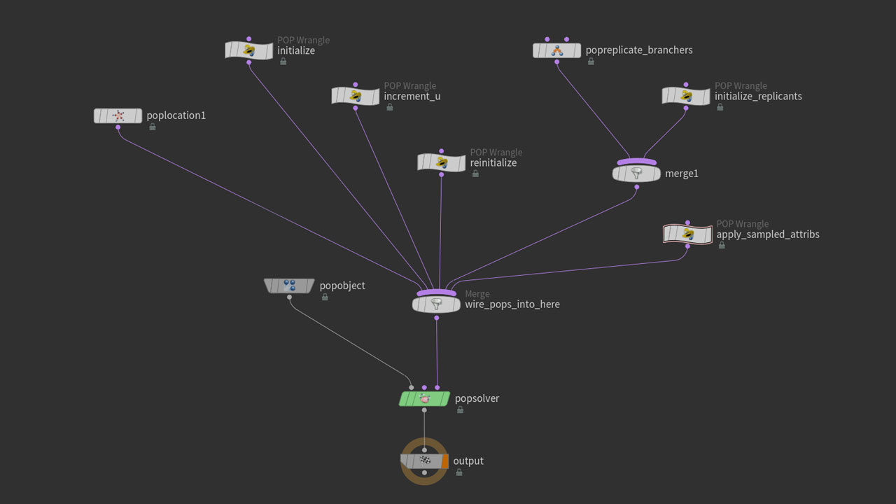
This is the POPs network. We have a POPLocation to source points at the root of the network, a clump of nodes that handle the prim traversal logic, and a couple of nodes for point replication (more on that later).

I should also note that the network of curves is the first input of the POPNet, with all wrangles inside having their input parms set accordingly. So any references to foo(0,...) inspect the original curve network.

So, to begin we spawn our points, and let the just born particles (defined with a group in the POPLocation) decide at random which of the prims connected to our root they travel along. This does that:

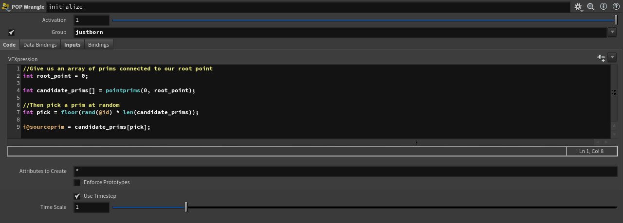
It’s worth noting that I’ve taken advantage of the fact the POPLocation defaults to spawn particles at the world origin, which happens to co-incide with single our root point. Fine for now, but something to keep in mind.

We retrieve an array of prims connected to our root point with the function primpoints(). From this array we pick a random prim, and then we primuv() our way along it. Hooyah.

So yes, we increment the U value that we’re using to sample the position on a prim, with a bit of per-particle speed randomization and adjusting for prim length as we go. Looking at this we could probably optimize away a few of the less prone-to-changing values were performance to become an issue, but for now:

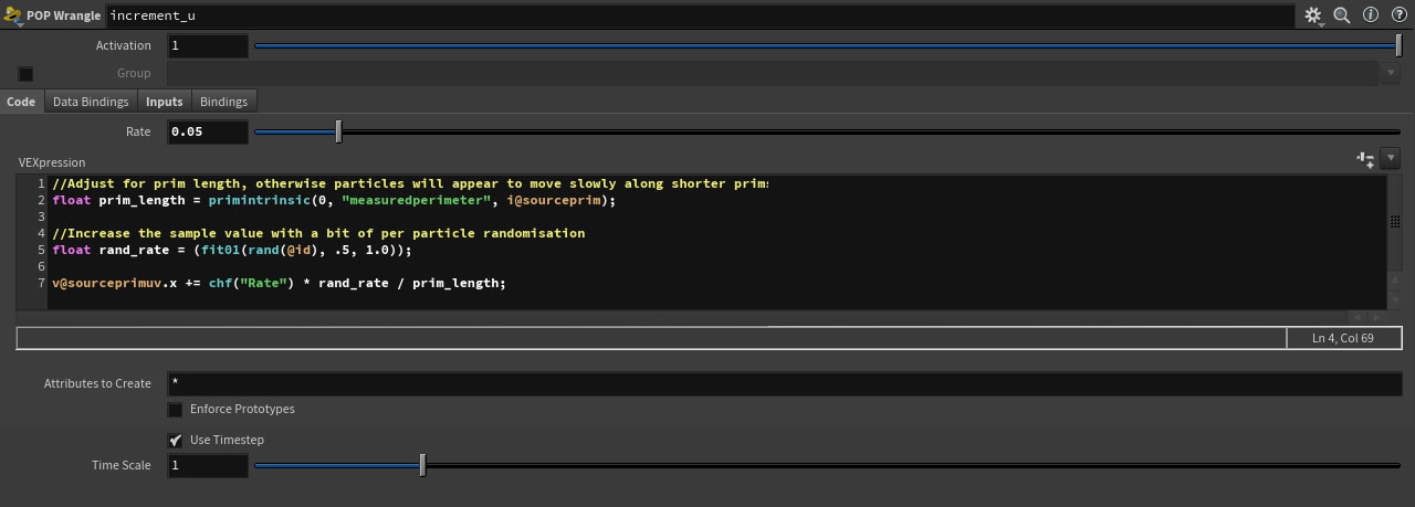
We now have all the information we need to sample the position, so let’s do that. We read the position, and a normal to orient the particle in the direction of the curve (created with an OrientAlongCurveSOP on the sampled curve network):

But what about when we arrive at a junction? We need to pick a new prim. Here’s how:

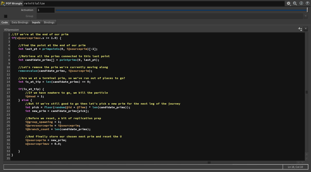
Any point with a U value greater than 1.0 has effectively moved beyond the end of the prim that it’s been travelling along, and so we can use this to find all the particles that need to choose their next prim. Now, in a similiar way as when picking our initial prim, we can look up all prims connected to the final point of our current prim, restarting the traversal by sampling the start of our new choice. We pick a new prim, we reset the uv, we continue onward.

The only additional consideration is what to do if the point is a terminal, if it has no connected prims where the U value is 1.0. Well… In which case there’s nowhere to go and the point must be killed off. Here I check this by asking for an array of connected prims, and then killing off the particle if that array is empty.

BUT. One more thing? As mentioned earlier, a common problem with branching structures is preserving particle density. As particles radiate outwards along generations of branches they will thin out, with each descision to go one way leaving an empty branches in all other directions.

So in this instance, rather than having a particle decide which branch to travel down, we will spawn sufficient particles in order to simaultaniously send something along each downstream prim. Why not.

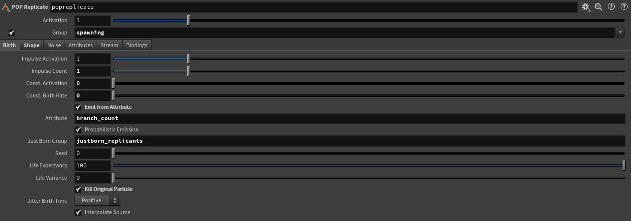
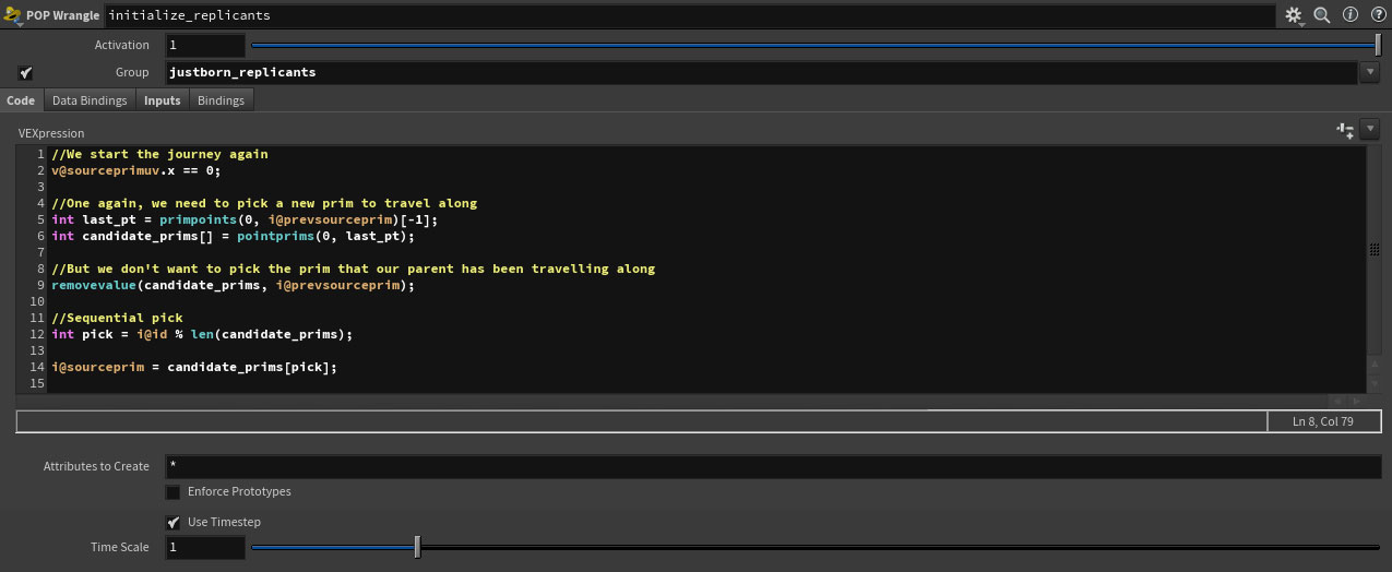
We use a branch_count attrib that dictates how many replicants will be spawned, and then we cycle though our array of connected prims to send the new particles on their way.

As a final tip. For easy dashed line geo, stuck the group syntax *:n into the “Cut Points” parm of a PolyCutSOP. Assuming you’ve sufficient resolution to support your desired look it’s an easy win.